Mix globally.
Propagate spatially.
Make the GPU work.
A small local update can build long-range interactions. GSPN keeps the image’s two-dimensional structure; GSPN-2 makes that scan efficient in practice.
A whole line moves together.
Instead of visiting every pixel in one long raster sequence, update a column in parallel, then advance to the next column. Repeat from four directions to collect context around each location.
A local step opens a wider view.
Each new column reads the three neighboring states in the preceding column. Repeated updates spread information through a growing cone.
Select another grid cell to inspect its context. The highlighted region shows which inputs can reach it, without explicitly building an all-pairs matrix.
A single direction is causal. The union of four directional cones covers the image. The grid illustrates dependency structure, not measured attention weights.
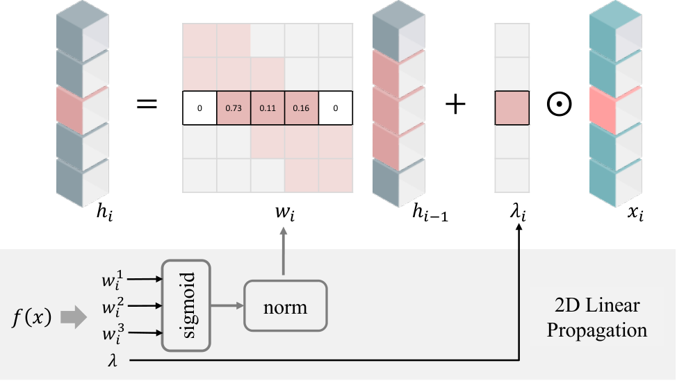
Three previous states.
One current input.
The equation and the program are the same story: collect nearby context from the preceding column, then add the gated input at this location.
H[h−1,w−1]G1H[h,w−1]G2H[h+1,w−1]G3H[h,w]Aw is the three-diagonal transition built from G1, G2 and G3.
Shift values down one row; a zero fills the missing top neighbor.
# X, B, G1, G2, G3: [batch, channels, height, width]
def gspn_forward(X, B, G1, G2, G3):
    H_minus1 = torch.zeros_like(X[..., 0])
    columns = []
    for w in range(X.shape[-1]):
        top = F.pad(H_minus1[..., :-1], (1, 0))
        bottom = F.pad(H_minus1[..., 1:], (0, 1))
        H_w = (B[..., w] * X[..., w]
               + G1[..., w] * top
               + G2[..., w] * H_minus1
               + G3[..., w] * bottom)
        columns.append(H_w)
        H_minus1 = H_w
return torch.stack(columns, dim=-1)Each tensor operation covers batch, channels and all rows. H_minus1 is a whole previous column. Zero padding supplies missing neighbors.
The first column starts from zero, so its output is simply B · X. This is a teaching rewrite of the full-width recurrence. The implementation uses a custom CUDA kernel ↓.
Gate normalization and the connection to attention
Apply sigmoid to the three incoming gates, then divide by their sum over valid neighbors. Each row of the propagation matrix sums to 1.
Aw 𝟙 = 𝟙 ⇒ (Aw ··· Aj) 𝟙 = 𝟙
Products of these transitions preserve the row sum as context travels farther. Input and output gates remain separate; the complete gated affinity need not sum to 1.
Paper wi = Aw here; λi = Bw. Paper ↗
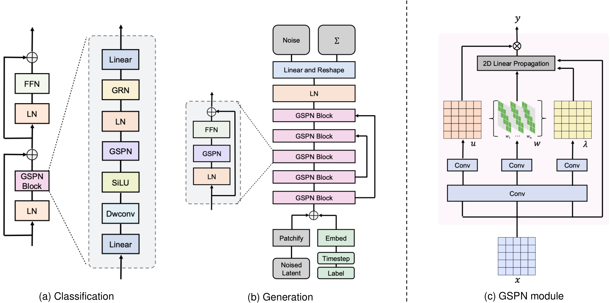
Linear work.
A shorter dependency chain.
Every pixel still needs an update. The gain is that an entire line can advance together, shortening the chain of dependent steps.
P = H × W
With C channels: O(P C) workOne new column per step
Square map: O(√P) depthAll rows can update together
Batch and channels add parallel work.This compares dependency structure, not measured implementations of Mamba or attention. O(√P) describes ideal scan depth with sufficient parallel resources. Total arithmetic and data movement remain linear in P for fixed channels and directions.
A GPU also pays for memory traffic, launches and scheduling. Shorter dependencies create an opportunity; the implementation determines how much of it becomes speed.
What about local chunks, prefix scans and full-block cost?
Independent chunks of length L reduce scan depth to L, but cut context at chunk boundaries. They do not reduce total pixel updates below linear work. Projection and channel-mixing layers add their own costs, commonly O(P C²).
Affine recurrences can be composed associatively. However, multiplying the three-diagonal spatial transitions widens their support; a generic matrix prefix scan loses the cheap three-neighbor representation. The issue is efficient representation, not a mathematical impossibility of parallel composition.
For rectangular maps, the four-direction dependency depth is O(max(H,W)). On fixed hardware, runtime is also limited by available compute, bandwidth and residency; it is not guaranteed to follow the ideal depth curve.
Keep the scan close to the data.
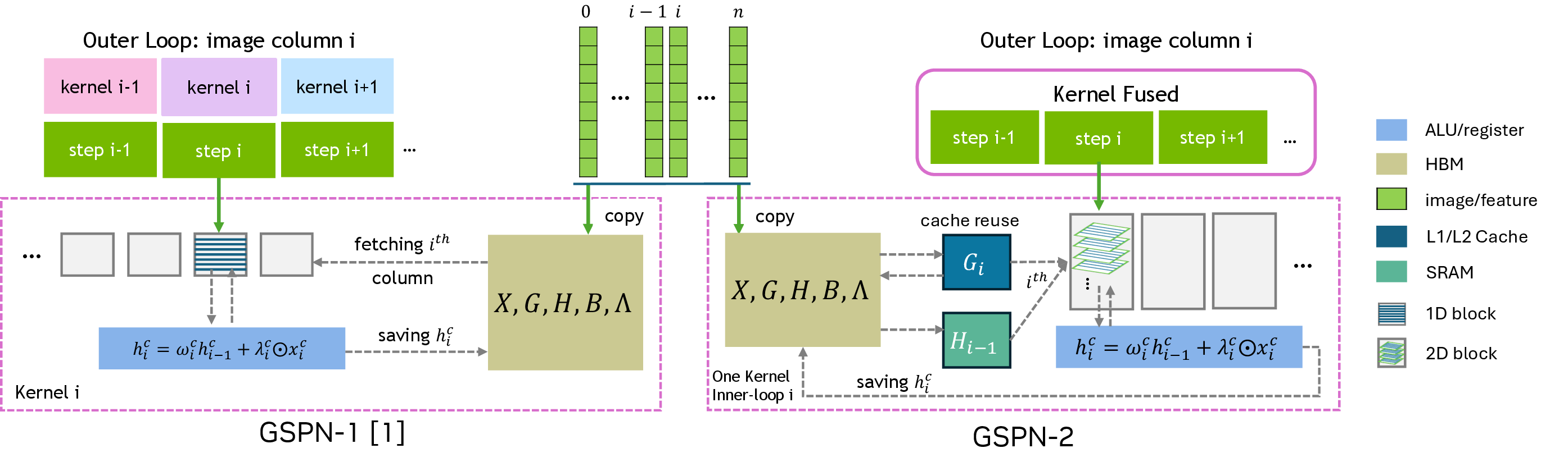
GSPN-2 moves the sequential loop inside the GPU kernel, then changes memory access so neighboring threads read neighboring values.
scalar_t h1_minus1 = g_data_1 * h_minus1_data_1;
scalar_t h2_minus1 = g_data_2 * h_minus1_data_2;
scalar_t h3_minus1 = g_data_3 * h_minus1_data_3;

scalar_t h_hype = h1_minus1 + h2_minus1 + h3_minus1;
scalar_t x_hype = b_data * x_data;
scalar_t h_data = x_hype + h_hype;

set_data_sf(H, num, channels, height,
            MIN_h, MAX_h, width, MIN_w, MAX_w,
n, c, h, w, h_data);Selected source statements, with boundary-aware loads omitted. The three h_minus1_data_* values are the upper-left, left and lower-left states; set_data_sf writes H.
Separate nonblocking streams can overlap the directional scans.
Read together. Fetch together.
In the original NCHW mapping, neighboring work items often access strided values. The hardware must gather data from separated regions.
Illustrative 8-thread layout; an actual CUDA warp has 32 threads. Address groups here explain locality, not a specific cache-line size or a measured transaction count.
not more arithmetic
The recurrence performs few arithmetic operations per value moved; coalescing improves useful memory throughput. Meanwhile, finite block residency makes excess work queue in waves—channel compression reduces that queued work.
Kernel implementation scope and occupancy
The original public CUDA source launches 512-thread blocks and one kernel per scan step. GSPN-2’s paper describes fusion, memory coalescing, selective on-chip caching and spatial/channel thread layout. Its public code link still points to the original repository, so the optimized kernel above is an architectural diagram, not a source-code excerpt.
Fusion must retain synchronization between dependent columns. Some large configurations still require multiple launches. The paper describes independent directional passes in separate nonblocking streams; this is not a claim that all four directions are one giant kernel.
The optimized operator’s reported profiles reach roughly 91–93% of peak global-memory throughput in the listed configurations; this is not a whole-model bottleneck claim. Shared memory is not automatically faster than hardware caching. Registers, shared memory and threads limit block residency, so neither a fixed “blocks per GPU” number nor unlimited channel parallelism explains actual throughput.
Original CUDA launcher ↗ · GSPN-2, §§4–5 ↗Fusion starts the job.
Memory layout makes the difference.
In the reported ablation, coalescing is the largest step. The final design also changes how channel work is represented and scheduled.
Arrange the computation so neighboring threads access neighboring addresses. This is the dominant gain in this reported configuration.
Selected milestones from GSPN-2’s A100 forward ablation. The final point also incorporates thread layout and channel compression. Timings are reported measurements, not a benchmark run on this page or an end-to-end model speedup. Original ablation figure ↗
Propagate a smaller channel state.
+ spatial scan
Share spatial affinities across channels and use a learned low-dimensional proxy to reduce the state that must be propagated.
Kernel engineering
Fusion and memory layout reorganize execution of the recurrence.
Model design
Shared affinities and channel compression change its parameterization. They require learned projections and should not be presented as a free, exact rewrite.
A fast kernel is only the beginning.
C-GSPN brings spatial propagation to foundation-scale vision encoders. It redesigns the surrounding block and learns from a strong attention-based teacher.
compact channels→Project up
Generate gates in the compact space and remove redundant projections around the scan. Optimize the block, not only its central kernel.
The teacher transfers useful representations; this is more than copying attention weights into a different formula.
Scope of the foundation-model claim
The follow-up is a distinct work, with compact latent propagation and cross-operator distillation. Its current hybrid encoder retains a small number of ordinary attention blocks. The propagation core has linear spatial work at fixed channels; that does not make the entire hybrid encoder asymptotically linear.
Operator, block and full-model speedups measure different things. Projections, normalization, feed-forward layers and retained attention all contribute to the end-to-end result.
C-GSPN manuscript ↗